By Eric Burden | December 9, 2020
In the spirit of the holidays (and programming), I’ll be posting my solutions to the Advent of Code 2020 puzzles here, at least one day after they’re posted (no spoilers!). I’ll be implementing the solutions in R because, well, that’s what I like! What I won’t be doing is posting any of the actual answers, just the reasoning behind them.
Also, as a general convention, whenever the puzzle has downloadable input, I’m
saving it in a file named input.txt.
Day 8 - Handheld Halting
Find the problem description HERE.
Part One - Lame-Boy
Maybe it’s just me and my fuzzy memories of high school Computer I class, but I’m getting a strong BASIC vibe from this puzzle. Here, we get a list of ‘instructions’ for a boot sequence on a handheld gaming device, whose sole purpose, it seems, is to jump around a bit before allowing the player to access their game. Probably teaching delayed gratification, or something. Anyway, let’s hurry up and parse some instructions!
Simulation Approach
The first approach we’ll use is to simulate running the instructions sequentially and ‘profiling’ the results to see what’s happened.
library(stringr)  # For `str_extract()`
library(purrr)    # For `map()`, `map2()`

test_input <- c(
  "nop +0",
  "acc +1",
  "jmp +4",
  "acc +3",
  "jmp -3",
  "acc -99",
  "acc +1",
  "jmp -4",
  "acc +6"
)
real_input <- readLines('input.txt')

# Helpful structure, a list containing one function per instruction type
# assigned by name
funs <- list(
  nop = function(accumulator, pointer, arg) {
    list(accumulator = accumulator, pointer = pointer + 1)
  },
  acc = function(accumulator, pointer, arg) {
    list(accumulator = accumulator + arg, pointer = pointer + 1)
  },
  jmp = function(accumulator, pointer, arg) {
    list(accumulator = accumulator, pointer = pointer + arg)
  }
)

# Helper function, given a vector of lines from the input (format 'acc +6'),
# returns # a nested list object where each list item represents a single
# instruction and each sublist item contains a [['fun']], which is the name of
# the instruction and an [['arg']], which is the argument for that line,
# ex. list(list(fun = 'acc', arg = 6), list(fun = 'nop', arg = -5))
parse_instructions <- function(funs, input) {
  fun <- str_extract(input, 'nop|acc|jmp')
  arg <- as.integer(str_extract(input, '[+-]\\d+'))

  result <- map2(fun, arg, list)
  result <- map(result, setNames, c('fun', 'arg'))
  result
}

# Main function, given a set of instructions (produced by
# `parse_instructions()`), runs the 'code' described and returns the result
# as a list containing the current `accumulator` value, the `pointer` to the
# current line in the instructions, a list of instruction line numbers in the
# order they ran as `run_lines`, and a flag for whether the instruction set
# was terminated by running all the instructions as `successfully_completed`.
profile_instructions <- function(instructions) {
  # These values are all in a list to make it easier to return the entire
  # package at the end
  profile <- list(
    accumulator = 0,
    pointer = 1,
    run_lines = numeric(0),
    successfully_completed = FALSE
  )

  # For each instruction in the list, follow that instruction and move
  # to the next instruction as appropriate
  while(profile$pointer <= length(instructions)) {
    current_line <- profile$pointer
    result <- with(
      instructions[[profile$pointer]],
      funs[[fun]](profile$accumulator, profile$pointer, arg)
    )

    # If we encounter a loop, return early with the profile
    if (profile$pointer %in% profile$run_lines) { return(profile) }

    # Update the profile
    profile$run_lines <- c(profile$run_lines, current_line)
    profile$accumulator <- result$accumulator
    profile$pointer <- result$pointer
  }

  # If the instructions run to completion, mark the profile as
  # `successfully_completed`
  profile$successfully_completed <- TRUE
  profile
}


instructions <- parse_instructions(funs, test_input)
final_profile <- profile_instructions(instructions)
answer <- final_profile$accumulator
To be transparent, this is the profile_instructions() function I ended up with
after getting to part two; when solving part one I hobbled by on a function that
only returned the last value of accumulator prior to exit. This is really the
way I should have started, though, since that profile list really gives some
helpful information back, and it provides everything we need to fix the
poor little boy’s issue (which we were definitely going to have to do in part
two no matter what).
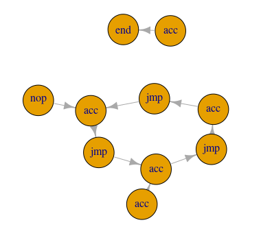
Graph Approach
A bit dissatisfied with the way part two turned out (code-wise), I felt there had to be a cleaner way to get at the answers to this puzzle. Well. there is another way, but I’ll leave it up to you to judge if it’s cleaner. Using a graph, we can represent the full path of our instruction set. By assigning the amount added to the accumulator with each step to the weight of the graph edges, we can check the value just prior to reaching the point where the program loops.
library(igraph)    # For all the graph-related functions
library(magrittr)  # For the %>% operator

instructions_to_graph <- function(instructions) {
  origins <- seq(length(instructions))        # Current instruction index
  names <- map_chr(instructions, ~ .x$name)   # Instruction name
  vals <- map_int(instructions, ~ .x$arg)     # Instruction value
  shifts <- ifelse(names == 'jmp', vals, 1)   # Amount to move by after instruction
  acc <- ifelse(names == 'acc', vals, 0)  # Amount to add to accumulator

  # Build a matrix where one column is the origins and the second column is the
  # represents the index of the next instruction in the sequence, determined
  # by the type and amount of the current instruction
  edge_matrix <- matrix(c(origins, origins + shifts), ncol = 2)

  # Make a graph! Converts the `edge_matrix` to a graph; assigns the 'name'
  # of the instruction to each vertex with a special name ('end') for the
  # vertex representing the space after the last instruction, assigns
  # the 'shift' of each instruction to each vertex as a `$shift` attribute,
  # assigns the amount added to the accumulator for each instruction to
  # each vertex as the '$acc' attribute
  graph_from_edgelist(edge_matrix) %>%
    set_vertex_attr('name', value = c(names, 'end')) %>%
    set_vertex_attr('shift', value = c(shifts, 0)) %>%
    set_vertex_attr('acc', value = c(acc, 0))
}

instructions <- parse_instructions(real_input)
instr_graph <- instructions_to_graph(instructions)
operation_path_vertices <- subcomponent(instr_graph, 1, mode = 'out')
answer <- sum(operation_path_vertices$acc)
The subcomponent() function takes a graph, a starting vertex (1 is the
first one), and a mode. 'out' means, basically, start with the given
vertex and move outwards. With these arguments, it returns a list of vertices
that are reachable from the starting vertex. We then sum the values of the
$acc component of each vertex returned to get the accumulator value
collected from traveling that path.
Part Two - Can We Fix It? (Yes, We Can!)
Simulation Approach
We knew we would end up here. Somehow, we’ve realized that there’s only one corrupted instruction. That’s great, because fixing two corrupted instructions would be way harder (I think). For the simulation approach, we profile the running of the instruction set (just like from part one) and iterate back through the rules that were executed in reverse order of execution, flipping instructions from ’nop’ to ‘jmp’. Each time we flip an instruction, we profile the instructions again to see if that fixed it.
# Main function, iterates backwards through the `run_lines` of the
# input profile, flipping 'nop's and 'jmp's when we come to them, checking
# the result by profiling again. If the program runs successfully, return
# the winning profile list early.
adjust_instructions <- function(fail_profile, instructions) {
  for (line in rev(fail_profile$run_lines)) {
    test_instructions <- instructions  # Copy the instructions before modifying
    current_fun <- instructions[[line]]$fun  # Get the instruction type

    # Flip 'jmp's to 'nop's, and vice versa
    if (current_fun == 'jmp') {
      test_instructions[[line]]$fun <- 'nop'
    }
    if (current_fun == 'nop') {
      test_instructions[[line]]$fun <- 'jmp'
    }

    new_profile <- profile_instructions(test_instructions)  # Test the change
    if (new_profile$successfully_completed) {
      print(paste0('It was ', line, '!'))  # Yells about the line that was fixed
      return(new_profile)
    }
  }

  new_profile
}

instructions <- parse_instructions(funs, real_input)
fail_profile <- profile_instructions(instructions)
new_profile <- adjust_instructions(fail_profile, instructions)
answer <- new_profile$accumulator
The print() command was 100% unnecessary, but I wanted to know which
instruction caused all these problems.
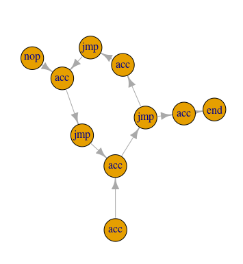
Graph Approach
The graph approach for part two felt a lot more complicated, but that probably
had more to do with my lack of familiarity with igraph than the complexity
of the problem. Actually, from a conceptual standpoint, the final logic is
pretty straightforward. Note that, unlike the simulation approach, we’re not
actually ‘flipping’ the ‘jmp’ to ’nop’ instructions and vice versa. Instead,
we’re just adding an edge to the ‘jmp’ and ’nop’ vertices, making them act
like both a ‘jmp’ and ’nop’ vertex at the same time. Neat! We could delete
the existing edge if we really wanted to, but it’s unnecessary in this case.
# Helper function, adds edges from 'jmp' vertices as if they were 'nop'
# vertices and adds edges to 'nop' vertices as if they were 'jmp' vertices
flip_instruction <- function(i, instr_graph) {
  v <- V(instr_graph)[[i]]
  if (v$name == 'jmp') {
    # Add an edge connecting to the next vertex in sequence
    mod_graph <- add_edges(instr_graph, c(i, i+1))
  }
  if (v$name == 'nop') {
    # Add an edge connection to the next vertex based on `shift` value
    mod_graph <- add_edges(instr_graph, c(i, i + v$shift))
  }
  mod_graph
}

get_path_to_end <- function(instr_graph) {
  # Get the vertex indices for the longest path starting at index 1,
  # AKA the indexes for all the vertices that can be reached from the
  # starting point
  steps <- subcomponent(instr_graph, 1, mode = 'out')  # Reachable vertices

  for (i in rev(steps)) {                # Stepping backwards
    if (instructions[[i]]$name %in% c('jmp', 'nop')) {
      # Flip the instruction at index `i` then check to see if there is a
      # `path` from the first vertex to the 'end' vertex. If there is,
      # return the list of vertices in that path.
      test_graph <- flip_instruction(i, instr_graph)
      path <- all_simple_paths(test_graph, 1, 'end', mode = 'out')
      if (length(path) > 0) { return(path[[1]]) }
    }
  }
}

instructions <- parse_instructions(real_input)
instr_graph <- instructions_to_graph(instructions)
path_to_end <- get_path_to_end(instr_graph)
answer2 <- sum(path_to_end$acc)
By default, all_simple_paths() would return all possible direct paths between
the two vectors, but since we’re changing only one edge at a time between
checks, we shouldn’t end up with more than one path. Plus, the problem told us
this would work, so…
Wrap-Up
This puzzle was fun for nostalgia’s sake, if nothing else. Also, graphs! After
wrapping up the simulation approach, I wasn’t completely satisfied, feeling that
there had to be a more elegant way to solve this one. I’m not sure that the
graph approach is more elegant, per se, but it was a lot of fun to reason
about. Plus, I learned a lot about igraph. Win-win! Note: It might be
possible for the graph approach, part two to simply ‘flip’ all the ‘jmp’ and
’nop’ vertices, calculate all the paths, and choose the shortest one. I say
might; it definitely works on the test input, but attempting it with the
real input was too much for my laptop to handle. Your mileage may vary.
If you found a different solution (or spotted a mistake in one of mine), please drop me a line!